Procedure 4: Forward Stepwise Logistic Regression

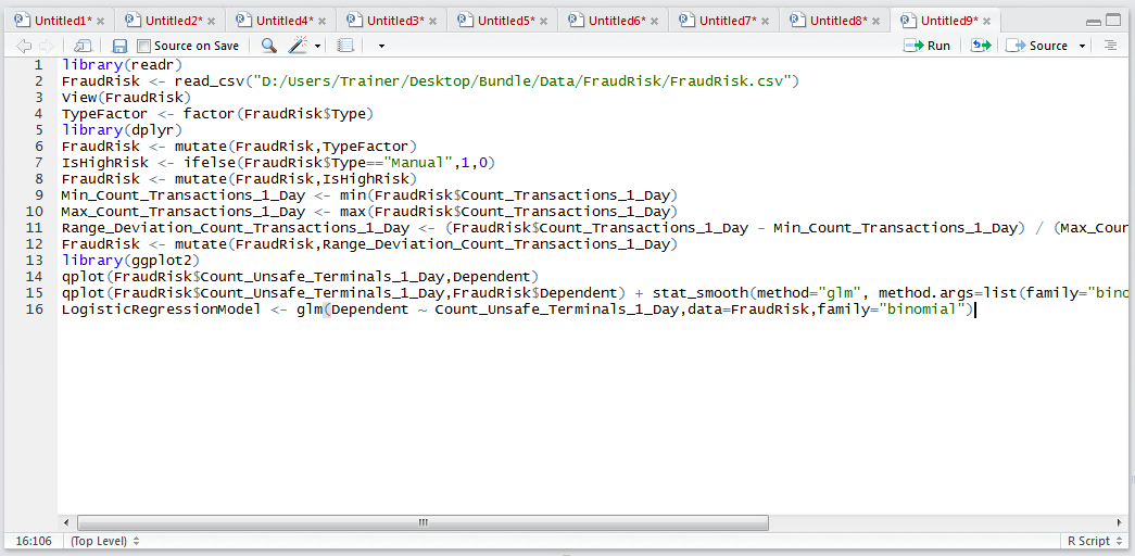
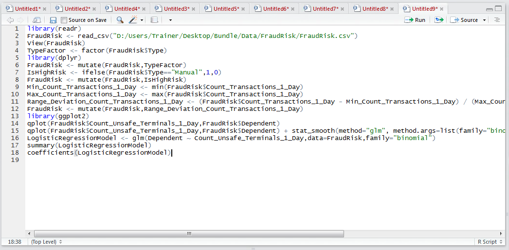
As procedure 97 alludes, whereas the linear regression function in R was lm(), the logistic regression function is glm(), with supplementary parameters specifying the family as being a binomial distribution (which is a stalwart distribution for classification problems). As in procedure 89 which create a linear regression model, the syntax is very similar to create a logistic regression model, albeit including the family argument:

LogisticRegressionModel <- glm(Dependent ~ Count_Unsafe_Terminals_1_Day,data=FraudRisk,family="binomial")

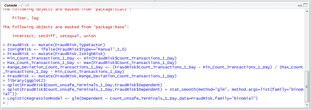
Run the line of script to console:

As with a lm() type model, the summary() function can return the model output:

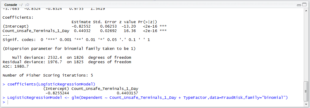
summary(LogisticRegressionModel)

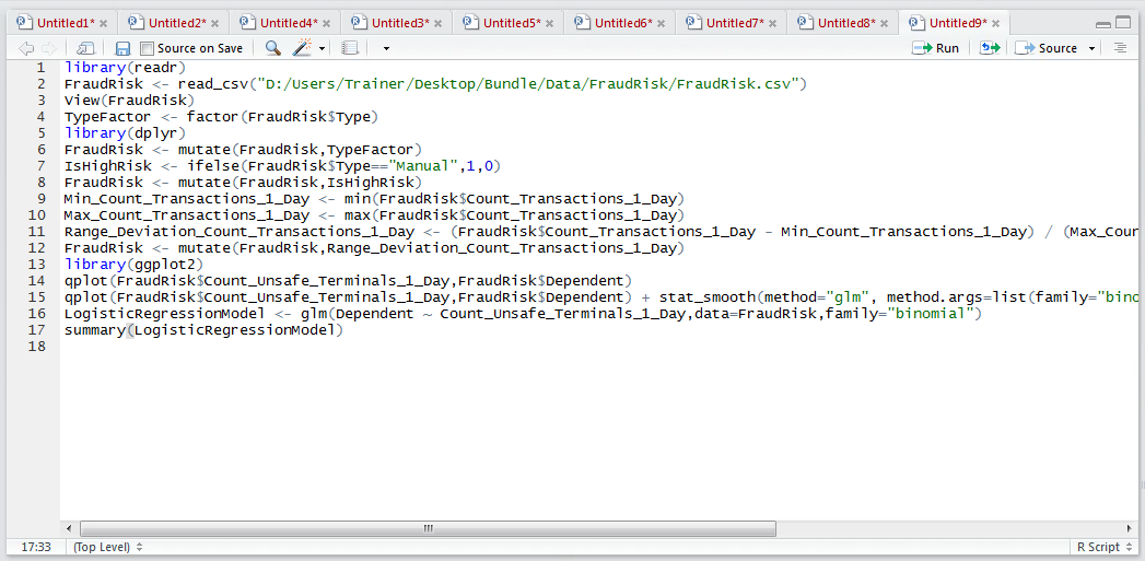
Run the line of script to console:

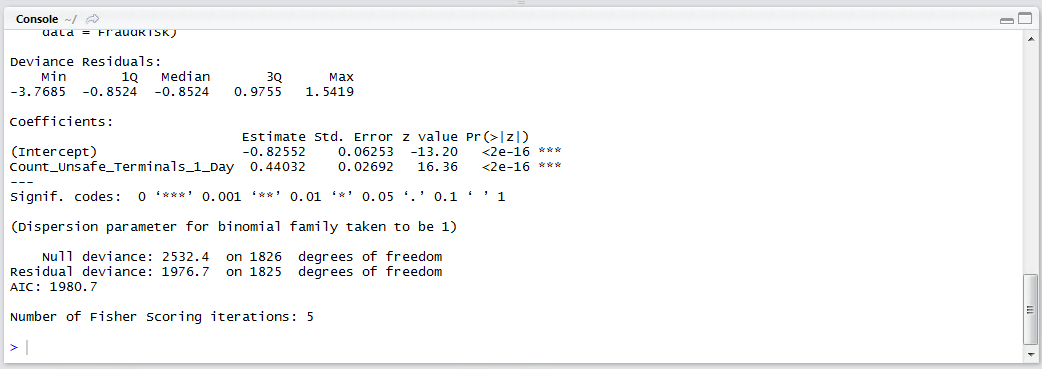
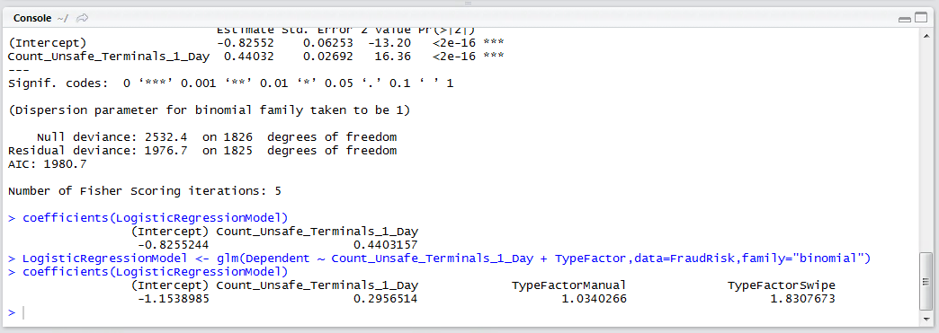
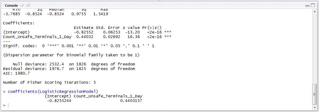
As with models created using the lm() function, the summary is somewhat inadequate to get the coefficients with correct precision, notwithstanding that the predict.glm() function will be used for recall:

coefficients(LogisticRegressionModel)

Run the line of script to console to output the coefficients for a manual deployment of the logistic regression model:

This procedure would naturally lead into a stepwise multiple logistic regression model, and in this example a factor as created in preceding procedures will be added with the assumption that it is the next strongest correlating factor:

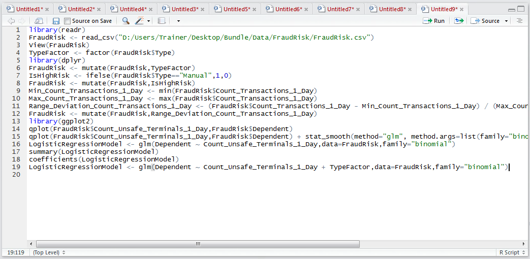
Run the line of script to console:

Write out the coefficients to observe the treatment of each different state inside the factor TypeFactor: